Setting Things Up

NOTE: The entire Python chapter is a shortened version of the tutorials in the psy111 course. Feel free to check this out in case you need more detailed explanations for some topics.

Installation

We will use Python through a software package called Conda. Conda is an environment management system that is widely used in the Python community and beyond. Conda allows you to create isolated environments, which you can think of as self-contained “boxes” that contain specific versions of Python and other packages required for different projects.

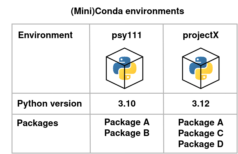
Fig. 1 Version management with Conda.

We will use a minimal version of Conda called Miniconda. This is a lightweight version of Conda that, unlike its bigger sibling Anaconda, comes without e.g. a graphical user interface. You can download and install it from here. Scroll down and select the suitable version for your operating system in the table. When installing Miniconda, please check the “Install for: All Users” checkbox to avoid potential issues with accessing Python packages.

In addition to Conda, we will also require a programming environment. If you do not have one installd already, you can download Visual Studio Code here. In addition to the default installation settings, we recommend you to check the “Open with code” checkboxes for easier usability later on.

The Python interpeter

After installing , search for the Anaconda Powershell Prompt (miniconda3) and open it. If you are on macOS or Linux, open the normal terminal. In all cases, you should see a (base) indicating that we have succesfully installed Miniconda and are in our base environment.

First, we will open the Python interpreter of our current base environment by typing python and then presssing enter. The Python interpeter will start and show you the current Python version, for example:

Python 3.12.4 | packaged by Anaconda, Inc. | (main, Jun 18 2024, 15:12:24) [GCC 11.2.0] on win32
Type "help", "copyright", "credits" or "license" for more information.
>>>

Simply put, the Python interpreter is the program that executes your Python code. It translates the written code into a form that the computer can understand and then runs it. Inside the interpreter we can write any kind of Python code, like printing a message:

>>> print("Hello World!")
Hello World!

While this works for simple commands, it is not really useful for more complicated tasks. These would usually be implemented in self-contained Python scripts or Jupyter notebooks. For now, let us exit the Python interpreter by typing quit() and pressing enter.

Conda environments

Remember that we use Conda to have isolated Python environments for our projects. So let’s start by creating a multiverse environment that is able to run all upcoming exercises (as well as create this entire book). Start by typing

conda create -n multiverse python==3.11

and confirm the installation with y when prompted to do so. This will then create the environment and already installs Python as well as some important packages. Afterwards, activate the environment by typing

conda activate multiverse

The (base)should now be changed to (multiverse), indicating that you have succesfully activated the new environment. You can then type

pip list

to display a list of all installed Python packages. As our environment is still new, this list is quite short. However, we are now ready to install any kind of Python package. Please to so for the comet-toolbox as well as the mne package, as we will require these two packages for the practical session tomorrow:

pip install comet-toolbox "mne[hdf5]"

If you then again type pip list, you will see that the list of installed packages now includes the NumPy. There are more things you can do with Conda, and if needed, you can refer to the cheatsheet for more information.

Python Scripts

We have previously used the Python interpreter to run simple Python code. However, you will ususally require a more organized way of running your code. For this, let’s open Visual Studio Code.

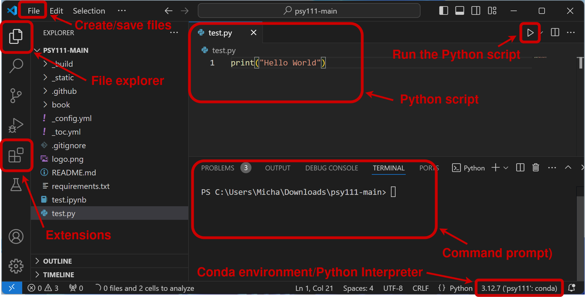
Fig. 2 Visual Studio Code.

First, navigate to the “Extensions” button in the left column and install the Python extension. Then, in the top left click on “File” -> “New file…” and select “Python file”. You will see that an empty file called “Untitled-1” was opened. We can save it by again clicking on “File” -> “Save”, or by pressing Ctrl + S (or Command + S on Mac). If you previously selected “Python file”, you can see that the .py file extension was automatically added to the file name (otherwise you can always do it manually).

You are now ready to write your Python script. As in the previous example, you can write

print("Hello World!")

and then run the Python script by pressing the run button at the top right. If you do this for the first time, VS Code will most likely promt you to select your Python interpeter at the bottom right. Here, you should now be able to see and select the previously created multiverse enviroment. If the terminal displays a yellow button even after loading the environment, hover your mouse over it and click “reload terminal”.

Jupyter notebooks

Python scripts (like the one you created in the previous section) are single files that run from top to bottom. Sometimes, for example if you have small projects that you would like to share with other, you might want to only have smaller blocks of code with text or images between them. In such cases, you can use Jupyter notebooks. These files contain cells for Python code as well as for text, so you can neatly format and share your code with others. We will also use these noteboks for the exercises in this seminar.

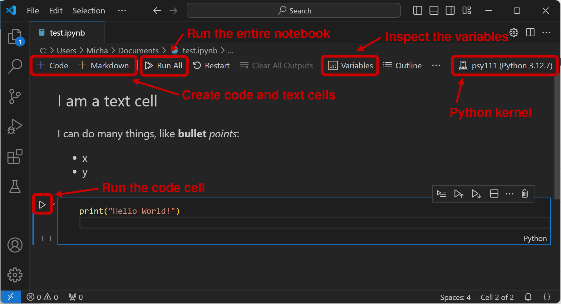
Fig. 3 Jupyter Notebooks.

To be able to use Jupyter notebooks, you need to install the Juypter extension (just like the previously installed Python extension). You can then create and use .ipynb files, which is short for “interactive python notebook”. Once you created such a notebook, you can add code cells with the + Code and text cells with the + Markdown buttons. The Python interpreter can again be selected from the multiverse environment by pressing the “Select Kernel” button at the top right of the script.

Code cells

Code cells can have any kind of Python code as an input. They will further also automatically print the last line:

a = 1
b = 2
a + b

3

Markdown cells

Markdown is a way of writing and formatting text. In fact, all the text in this book is written in Markdown (or to be more specific with MyST Markdown, which is an extension to Markdown). As a start, you can use the cheatsheet to learn about the basic syntax. You will be able to explore this in the upcoming exercises.

Testing your Python Environment

Create either a standard .py Python script or a .ipynb Jupyter Notebook and run the following code to test your environment:

# Test the imports
import comet
import mne

# Create an example plot
import numpy as np
from matplotlib import pyplot as plt
from matplotlib.collections import LineCollection

colors = ["indigo", "blue", "green", "yellow", "orange", "red"]

theta = np.linspace(0, np.pi, 36)
radii = np.linspace(4, 5, num=len(colors))
arcs = [np.column_stack([r * np.cos(theta), r * np.sin(theta)]) for r in radii]

fig, ax = plt.subplots()
ax.set_xlim(-6, 6)
ax.set_ylim(0, 6)
ax.set_aspect("equal")

line_collection = LineCollection(arcs, colors=colors, linewidths=4)
ax.add_collection(line_collection)
ax.text(0, 1, "Welcome to the PuG 2025\n Multiverse Workshop!", fontsize=14, ha='center')

plt.show()

Summary

You can use Python in different ways:

• Through standard Python scripts (.py files)

• Through interactive Jupyter Notebooks (.ipynb files)

You can use Conda to manage your Python environments. You can:

• Create environments with conda create -n <env_name>

• Switch environments with conda activate <env_name>

• Install packages using pip install inside the environment